반응형
< Web 화면에 차트그리기 1 >
# 기본적으로 모든 코드들은
def main() :
if __name__ == '__main__' :
main()
ㄴ 이 기본형식 안에서 쓰여저야 실행된다. 혹시 실행이 되지 않을경우 하단에 마무리 코드를 적지 않았는지 확인!
# 웹 화면에 실행 확인은 생성한 파일명이나 혹은 연동한 app을 서버로 실행하여야 함.
# 터미널을 cmd로 열어 & streamli lit run 실행시킬서버명칭.py 로 실행후 always rerun 후 확인
< app9.py로 작성 >
import streamlit as st
import pandas as pd
import matplotlib.pyplot as plt
import seaborn as sb
# 차트를 그려낼 데이터 가져오기
def main() :
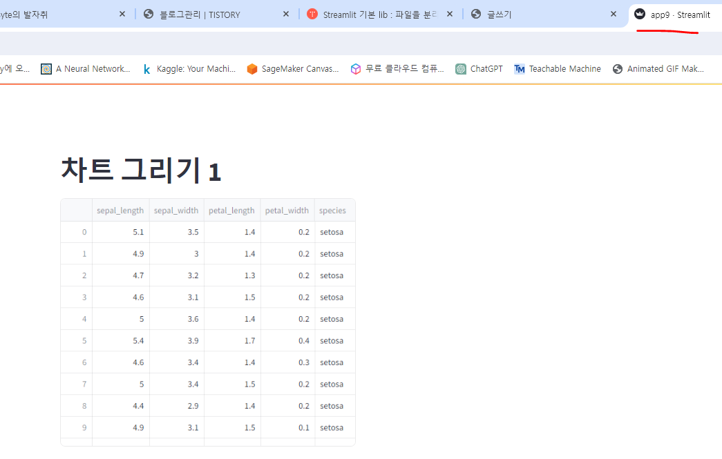
st.title('차트 그리기 1')
df = pd.read_csv('./data/iris.csv')
st.dataframe(df)
# 기본적으로 streamlit으로 차트를 그리기 위해서 차트 영역을 만들어주어야 한다.
# fig1, fig2, fig3
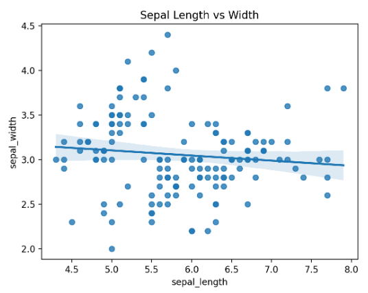
# sepal_length 와 speal_width 의 관계를 차트로 나타내시오.
# 두컬럼간의 관계이면 당연히 scatter (plt 스케터, 시본의 스케터플롯 등) 이다 라고 외워야 한다.
fig1 = plt.figure()
plt.scatter(data= df, x='sepal_length', y='sepal_width')
plt.title('Sepal Length vs Width')
st.pyplot(fig1)
fig2 = plt.figure()
sb.scatterplot(data= df, x='sepal_length', y='sepal_width')
plt.title('Sepal Length vs Width')
st.pyplot(fig2)
fig3 = plt.figure()
sb.regplot(data= df, x='sepal_length', y='sepal_width')
plt.title('Sepal Length vs Width')
st.pyplot(fig3)

# sepal_length 로 히스토그램을 그린다.
# bins 의 갯수는 20개로.
fig4 = plt.figure()
plt.hist(data= df, x='sepal_length', bins=20, rwidth=0.9)
plt.title('Histogram')
plt.xlabel('sepal_length')
plt.ylabel('count')
st.pyplot(fig4)

# sepal_length 히스토그램을 그리되,
# bins 의 갯수를 10개와 20개로
# 두개의 차트를 수평으로 보여주세요.
fig5 = plt.figure(figsize=(10, 4))
plt.subplot(1, 2, 1)
plt.hist(data= df, x='sepal_length', bins=10, rwidth=0.9)
plt.title('Histogram')
plt.xlabel('sepal_length')
plt.ylabel('count')
plt.subplot(1, 2, 2)
plt.hist(data= df, x='sepal_length', bins=20, rwidth=0.9)
plt.title('Histogram')
plt.xlabel('sepal_length')
plt.ylabel('count')
st.pyplot(fig5)

# 판다스의 데이터프레임의 차트도 그릴수 있다.
# species 는 각각 몇개인지 나타내시오.
print(df['species'].value_counts())
# 위의 결과를 바차트로 나타내시오.
fig6 = plt.figure()
df['species'].value_counts().plot(kind='bar')
st.pyplot(fig6)
# sepal_length 컬럼을 히스토그램으로 나타내시오.
fig7 = plt.figure()
df['sepal_length'].hist()
st.pyplot(fig7)

# df 의 상관계수를 구해서, 차트로 표시!
fig8 = plt.figure()
df_corr = df.corr(numeric_only= True)
sb.heatmap(data=df_corr, vmin= -1, vmax=1, annot=True, fmt='.1f')
st.pyplot(fig8)

### app9.py 전체 코드 ###
import streamlit as st
import pandas as pd
import matplotlib.pyplot as plt
import seaborn as sb
def main() :
st.title('차트 그리기 1')
df = pd.read_csv('./data/iris.csv')
st.dataframe(df)
# sepal_length 와 speal_width 의 관계를 차트로 나타내시오.
# 두컬럼간의 관계이면 당연히 scatter (plt 스케터, 시본의 스케터플롯 등) 이다 라고 외워야 한다.
fig1 = plt.figure()
plt.scatter(data= df, x='sepal_length', y='sepal_width')
plt.title('Sepal Length vs Width')
st.pyplot(fig1)
fig2 = plt.figure()
sb.scatterplot(data= df, x='sepal_length', y='sepal_width')
plt.title('Sepal Length vs Width')
st.pyplot(fig2)
fig3 = plt.figure()
sb.regplot(data= df, x='sepal_length', y='sepal_width')
plt.title('Sepal Length vs Width')
st.pyplot(fig3)
# sepal_length 로 히스토그램을 그린다.
# bins 의 갯수는 20개로.
fig4 = plt.figure()
plt.hist(data= df, x='sepal_length', bins=20, rwidth=0.9)
plt.title('Histogram')
plt.xlabel('sepal_length')
plt.ylabel('count')
st.pyplot(fig4)
# sepal_length 히스토그램을 그리되,
# bins 의 갯수를 10개와 20개로
# 두개의 차트를 수평으로 보여주세요.
fig5 = plt.figure(figsize=(10, 4))
plt.subplot(1, 2, 1)
plt.hist(data= df, x='sepal_length', bins=10, rwidth=0.9)
plt.title('Histogram')
plt.xlabel('sepal_length')
plt.ylabel('count')
plt.subplot(1, 2, 2)
plt.hist(data= df, x='sepal_length', bins=20, rwidth=0.9)
plt.title('Histogram')
plt.xlabel('sepal_length')
plt.ylabel('count')
st.pyplot(fig5)
# 판다스의 데이터프레임의 차트도 그릴수 있다.
# species 는 각각 몇개인지 나타내시오.
print(df['species'].value_counts())
# 위의 결과를 바차트로 나타내시오.
fig6 = plt.figure()
df['species'].value_counts().plot(kind='bar')
st.pyplot(fig6)
# sepal_length 컬럼을 히스토그램으로 나타내시오.
fig7 = plt.figure()
df['sepal_length'].hist()
st.pyplot(fig7)
# df 의 상관계수를 구해서, 차트로 표시!
fig8 = plt.figure()
df_corr = df.corr(numeric_only= True)
sb.heatmap(data=df_corr, vmin= -1, vmax=1, annot=True, fmt='.1f')
st.pyplot(fig8)
if __name__ == '__main__' :
main()
다음 게시글로 계속
728x90
반응형
'DASHBOARD APP 개발 > Streamlit Library' 카테고리의 다른 글
| Streamlit 기본 문법 모음 & 환경 세팅 전체 정리 (0) | 2024.05.08 |
|---|---|
| Streamlit 기본 lib : Web 화면에 차트그리기 2 (스트림릿의 내장 차트 함수와 유명한 라이브러리인 plotly 차트) (0) | 2024.05.07 |
| Streamlit 기본 lib : 파일을 분리해서 개발하는 방법 (0) | 2024.05.07 |
| Streamlit 기본 lib : Web화면에서 이미지, csv 파일 업로드 하기 (0) | 2024.05.07 |
| Streamlit 기본 lib : Web화면에서 유저한테 숫자, 문자, 시간, 색 입력받기 (0) | 2024.05.07 |